Mapping Public Transit Networks

A few months ago the worldwide public transit tracker developed by geOps and the University of Freiburg, TRAVIC, went online. To visualize the vehicle movements, we use an approach that combines static timetable data and real-time delay information (both defined in the GTFS) and calculates vehicle positions by interpolating this data.

For this approach to yield reasonable good results, we not only need the temporal progression of a vehicle trip (in the form of arrival and departure times), but also the spatial one. While the GTFS defines the exact coordinates of stops as a required field, the routes vehicles take through the network (shapes) are an optional information. This means that many feeds only contain enough information to do a very rough visualiziation where vehicles fly from one stop to the next, neither following street nor rail networks.

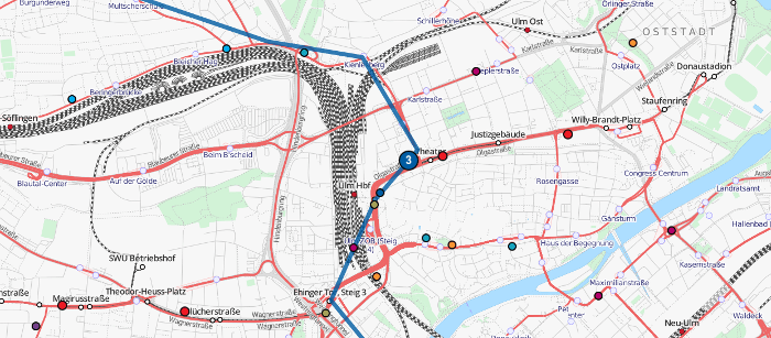
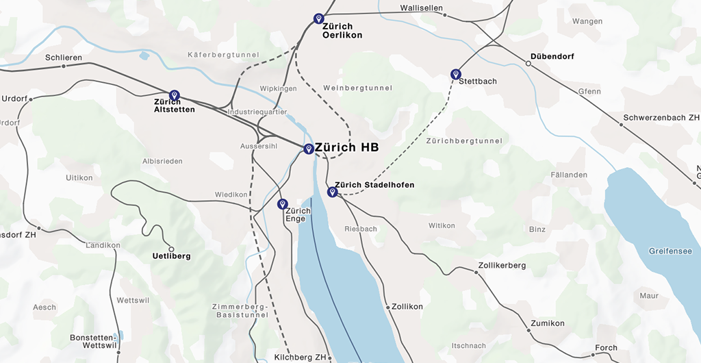
By the time we decided to include the public transportation network of switzerland into TRAVIC we could no longer dispose the problem as a minor flaw. However, apart from station positions, the raw data we use to convert our GTFS feeds from does not contain any spatial information.

Extracting vehicle routes from geo-data

Attempts to compare the set of railway relations in OpenStreetMap to the set of station-to-station geometries from GTFS feeds (e.g. via a Fréchet-Distanz) were fruitless. A look at the street network (already transformed into a graph) of Zurich gives a hint of the complexity of extracting bus routes from even a very small area.

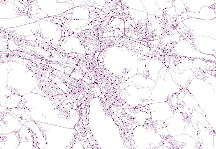
Our approach generates vehicle route shapes by using iterative shortest-path calculation on the public transit network. Naturally, a vehicle does not always take the "optimal" route from one station to another. In fact, for railway networks, naïve shortest paths are very often the wrong ones. We need good heuristics to be able to distingiush likely from unlikely vehicle routes.

The general flow of our approach looks like this:

1. built a graph from rail or road geometries, sort in stops from GTFS
2. look at every trip in the GTFS feed, calculate the shortest path between every two succeeding stations
3. check for plausibility
4. filter and compress shapes to avoid redundancy

In the following, we will illustrate each of the steps mentioned above.

1. Graph

More than often, the geographical reference data only consists of a loose collection of line geometries. To do shortest-path calculation on the data we need to transform these geometries into a topologically valid graph and connect it to the schedule data. Thus, we clean the reference data from unintentional gaps in the network.

To establish a connection between the schedule data and the spatial reference data, we insert the stops referenced in the timetable data into the graph. This step is far from trivial. In general, we cannot, for example, just take existing stations defined in the OpenStreetMap data and correlate them to the stations defined in the GTFS feed. First, we want to be able to handle geospatial reference data without any stop information. Second, the correlation between schedule stops and reference data stops is, in general, difficult. Especially for busses in rural areas, OpenStreetMap lacks many stops. Additionally, if stops are available, they are more than often orphanaged and without connection to any line geometries. Even in metropolitan areas where stops are usually defined comprehensively, it is difficult to find the node in the geospatial data that corresponds to the station defined in the schedula data. A correlation based solely on distance will fail because of the sheer station densitity on highly populated areas. Only very, very few stations in OSM are provided with IDs that correspond to an ID in the GTFS feed. The difficulties that arise when trying to correlate two stations based on their names shows the following (fictitious) example of possible notations of a bus station (called "Giess Street") in Germany.

• Gießstraße
• Gießstrasse
• Giessstrasse
• Gießstr.
• Giessstr.
• Mühlenheim, Gießstraße
• Großdorf-Mühlenheim, Gießstraße
• Großdorf (Baden), Mühlenheim, Gießstraße
• Großdorf, Baden, Mühlenheim, Gießstr.
• Gießstraße (Mühlenheim)
• etc.

Stop name notation in OSM or in the GTFS does not follow any schema.

Because the correct insertion of stops into the geospatial data is crucial for the quality of our results, we determine the position of a station in our graph using a multistage approach.

First, an area search determines the nodes in the reference data that are marked as 'stop' and are within a fixed radius to the position of the schedules stop. We insert these nodes into a priority queue, sorted by criterias equality of station id, distance and similarity of station name. If there is no node marked as a station in the near area (usually around 500 meters), we analyse the surrounding edges. We also insert them into a priority queue, based on criterias distance to schedule stop (based on the projected position of the schedule stop onto the edge), the order of the edge (for example residencial road vs. highway) and the vehicle type that is defined in the reference data to travel on this edge. The schedule station will be snapped onto the best matching edge. Following this approach, in the case of OSM data, a bus station will be snapped onto a main street that belongs to a OSM bus relation with a much higher probability then on a small alley.

In most cases, however, a station consists of multiple stop points. At first glance this seems to be a cosmetical problem. Even in bus networks, though, a correct placement of secondary stations is crucial and is tightly connected to the topological correctness of the graph. The following example illustrates this.

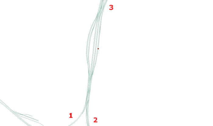
Although the station (red dot) is snapped correctly on one of the tracks, it is impossible to reach the station when comming from string 1. In bus networks, a similar problem occurs on roads with multiple lanes that are marked as one-way roads, respectively. If the station in the opposite direction is missing, the bus has to take huge detours during the calculation of the shortest path to reach the station heading in the right direction.

To cover these cases, we do not only take the best stop from the priority queue as described above, but a (predefined) number of possible candidates.

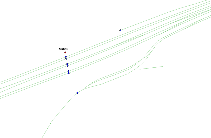
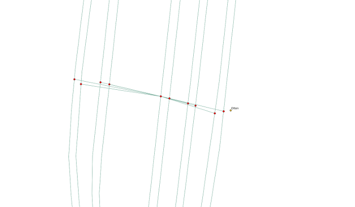
These candidates are now connected to the primary station by dummy edges. This means that we are allowing a train to switch tracks in stations. Without these special edges a successful shortest path calculation would only be possible in very few cases. However, these special edges are also the main source of outliers in our results. The figure below shows the station of Olten in Switzerland with the special edges included.

2. Shortest-Path-Algorithm

After the graph was generated, we iterate through each trip in the schedule data and calculate the shortest path between two succeeding stations. "Shortest path" has to be understood symbolically here. It is the "cheapest" path. The calculation of edge costs is done dynamically and is based on heuristics. We will present two exemplary heuristics here.

Full turns

Usually, trains don't do full turns out of stations. One of the most important heuristics is to punish full turns for rail-bound methods of transportation, but also for busses. This is done by dynamically adding edge costs based on the entry and exit angle at nodes.

OSM-Relation snapping

For most methods of transportation, OpenStreetMap holds plenty of relations. Most of them contain even the vehicle's line number. To prevent the loss of this useful information, edge costs are dynamically reduced if the edge belongs the a relation that matches the vehicle the shortest path is currently searched for. Because of this, schedule routes that have counterparts in OSM relations usually follow the exact route defined for this relation in OSM.

3. Plausibility

After a vehicle shape generation is completed, the shape is checked for plausibility. This is done by comparing the length of the vehicle route as the crow flies to the length of the found vehicle shape. Additionally, the average velocity needed to get from one station to another on time is calculated. For huge deviations from the real-world vehicle route, the required velocity is usually > 1,000 km/h. Thus, the deviation can safely be identified and configuration parameters can be adjusted.

4. Compression and Redundancy Avoidance

Vehicles in public transit networks usually share a common route. It makes little sense to generate shapes for all trips of a bus line if all of them follow the exact same route. This is why we do a comparision based on the station sequence, the method of transportation and the line number to find vehicle routes that have been previously calculated before starting a new calculation. Additionally, to cover the case when vehicles of different lines or even of different MOTs share a common route, we compare the found paths to the already found ones. This comparision also tries to cover cases where a vehicle uses a connected subset of an already existing path.

Results

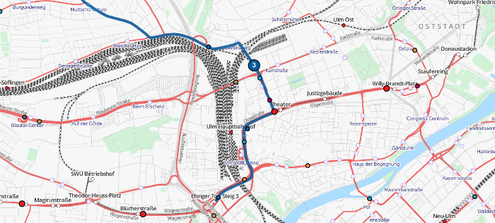
Using the approach described above we calculated the vehicle routes for the complete public transport network (busses, trams, subways, trains, ferries) of Germany and Switzerland. The results (except the ones for Germany which are currently not available due to missing data after the timetable change) are visible on http://tracker.geops.de.

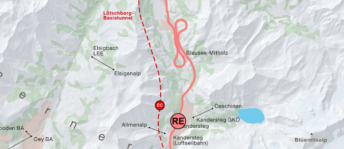
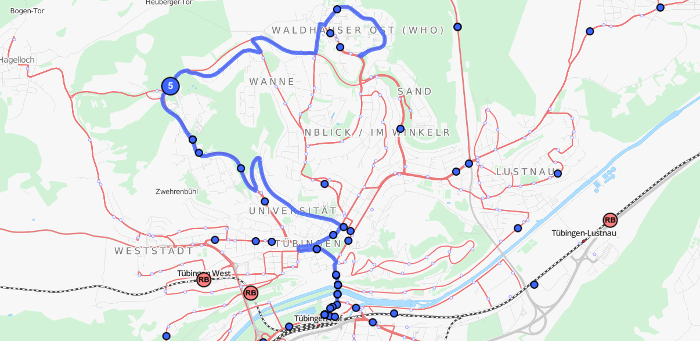
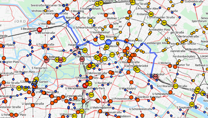
It is also possible to generate and output either the complete or the filtered network, based on the schedule and complete with line numbers for single areas or whole countries. The figure below shows the generated bus network of the city of Zurich.

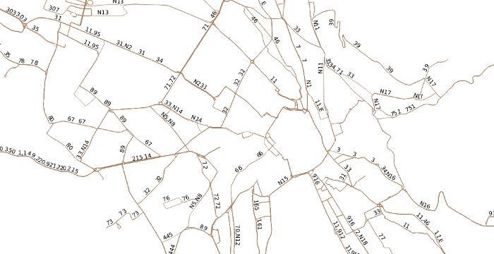
Each geometry corresponds to one or more vehicles travelling on this route through the network. We can handle requests like "which route does the bus serving line 2 take on August 22nd, starting a stop X at 7:20?"'.

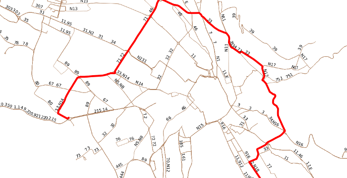
The shape generation is not restricted to OpenStreetMap as the geospatial reference data. In principle, each data source that can be transformed into a geo referenced graph can be used (e.g. geometries from a PostGIS database). For the transit tracker on the Swiss federal railway's Trafimage map we used shapefiles to generate vehicle shapes for different generalization levels.